連立一次方程式の解法の1つに,「クラメルの公式」というものがあります。これは,連立一次方程式の解を,行列式で表そうとするものです。これについて,その内容と具体例・証明を詳しく解説しましょう。
クラメルの公式
n 個の変数, n 個の式がある1次連立方程式
\begin{cases} a_{11} x_1+a_{12}x_2+\dots + a_{1n} x_n = b_1 \\ a_{21} x_1+a_{22}x_2+\dots + a_{2n} x_n = b_2 \\ \dots \\ a_{n1} x_1+a_{n2}x_2+\dots + a_{nn} x_n = b_n\end{cases}
は,行列を用いて
\begin{pmatrix} a_{11} & a_{12} &\dots &a_{1n} \\ a_{21} & a_{22} &\dots &a_{2n} \\ \vdots & \vdots &\ddots &\vdots \\ a_{n1} & a_{n2} &\dots &a_{nn} \end{pmatrix} \begin{pmatrix} x_1 \\ x_2 \\ \vdots \\x_n\end{pmatrix} = \begin{pmatrix} b_1 \\ b_2 \\ \vdots \\b_n\end{pmatrix}
と表すことができます。これは,
\begin{aligned} A&= (\boldsymbol{a_1}, \boldsymbol{a_2}, \dots, \boldsymbol{a_n}) \\ &= \begin{pmatrix} a_{11} & a_{12} &\dots &a_{1n} \\ a_{21} & a_{22} &\dots &a_{2n} \\ \vdots & \vdots &\ddots &\vdots \\ a_{n1} & a_{n2} &\dots &a_{nn} \end{pmatrix}, \\ \boldsymbol{x} &= \begin{pmatrix} x_1 \\ x_2 \\ \vdots \\x_n\end{pmatrix} ,\; \boldsymbol{b} = \begin{pmatrix} b_1 \\ b_2 \\ \vdots \\b_n\end{pmatrix} \end{aligned}
とおくと,
A\boldsymbol{x} =\boldsymbol{b}
のようにかけます(このとき, A を係数行列といいます→係数行列・拡大係数行列とは)。
このときの解 \boldsymbol{x} に関連する公式で,クラメルの公式というものがあります。それが,以下です。
定理(クラメルの公式; Cramer’s rule)
連立1次方程式 A \boldsymbol{x} = \boldsymbol{b} について, A が正則行列(可逆行列)であるとする。このとき,この連立方程式の解はただ一組で,
\boldsymbol{x} = A^{-1} \boldsymbol{b}
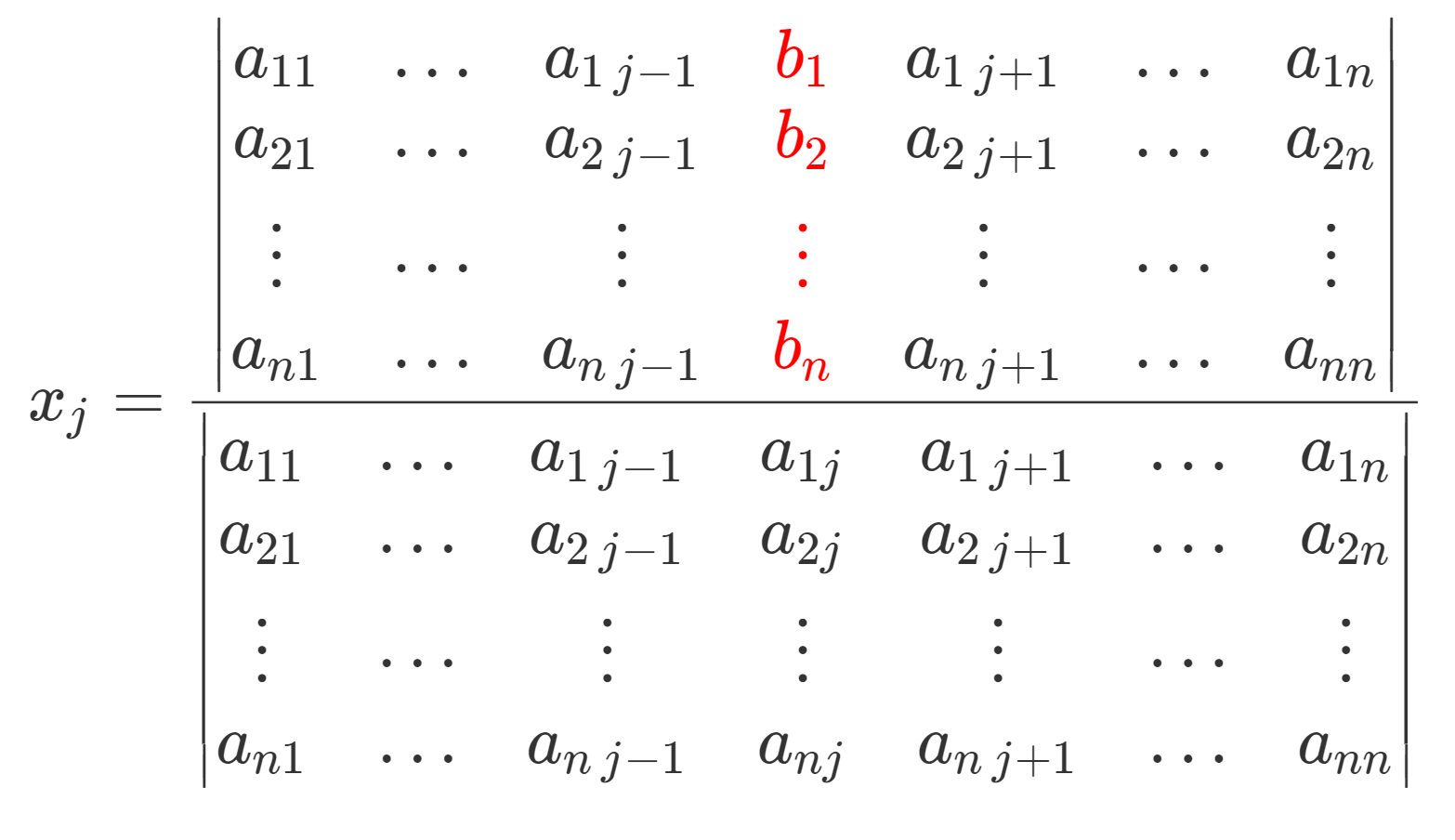
とかけるが,これは A_j = (\boldsymbol{a_1},\dots, \boldsymbol{a_{j-1}}, \textcolor{red}{\boldsymbol{b}}, \boldsymbol{a_{j+1}},\dots, \boldsymbol{a_n}) とおくと,
\color{red} x_j = \frac{\det A_j}{\det A},\quad 1\le j\le n
とも表せる。
前半部分は,両辺左から A^{-1} をかけると考えると,明らかです。
後半の部分がクラメルの公式です。 A_j は, A の第 j 列を \boldsymbol{a_j} から \boldsymbol{b} に置き換えたものになります。詳しく書くと,
A_j = \begin{pmatrix} a_{11} &\dots & a_{1\,j-1} & \textcolor{red}{b_1} &a_{1\,j+1} &\dots & a_{1n} \\ a_{21} &\dots & a_{2\,j-1} & \textcolor{red}{b_2} &a_{2\,j+1} &\dots & a_{2n} \\ \vdots & \cdots & \vdots & \textcolor{red}{\vdots} & \vdots & \cdots & \vdots \\ a_{n1} &\dots & a_{n\,j-1} & \textcolor{red}{b_n} & a_{n\,j+1} &\dots & a_{nn} \end{pmatrix}
ですね。これを用いて詳細に解をかくと,
x_j =\frac{ \begin{vmatrix} a_{11} &\dots & a_{1\,j-1} &\textcolor{red}{ b_1} &a_{1\,j+1} &\dots & a_{1n} \\ a_{21} &\dots & a_{2\,j-1} & \textcolor{red}{b_2} &a_{2\,j+1} &\dots & a_{2n} \\ \vdots & \cdots & \vdots & \textcolor{red}{\vdots} & \vdots & \cdots & \vdots \\ a_{n1} &\dots & a_{n\,j-1} & \textcolor{red}{b_n} & a_{n\,j+1} &\dots & a_{nn} \end{vmatrix} }{ \begin{vmatrix} a_{11} &\dots & a_{1\,j-1} & a_{1j}&a_{1\,j+1} &\dots & a_{1n} \\ a_{21} &\dots & a_{2\,j-1} & a_{2j}&a_{2\,j+1} &\dots & a_{2n} \\ \vdots & \cdots & \vdots & \vdots & \vdots & \cdots & \vdots \\ a_{n1} &\dots & a_{n\,j-1} & a_{nj} & a_{n\,j+1} &\dots & a_{nn} \end{vmatrix} }
となります。
注意ですが,クラメルの公式は,非常に計算が煩雑であり,実運用上はあまり有用ではありません。あくまで「理論値」として,この公式が役立つ場面がある,という程度の認識でいてください。
行列を用いて連立一次方程式を解く現実的な方法は,以下で解説しています。
クラメルの公式の例題
「実運用上はあまり有用でない」と述べましたが,一応例題を挙げてみましょう。計算の大変さが分かると思います。
例題
連立一次方程式 \begin{cases} 2x_1+3x_3+4x_3= 1 \\ x_1+4x_2-2x_3 = 3 \\ x_1-x_3 = 2\end{cases} の解 \begin{pmatrix} x_1 \\x_2 \\x_3\end{pmatrix} をクラメルの公式を使って求めよ。
求めてみましょう。
解答
A = \begin{pmatrix} 2& 3 & 4 \\ 1 & 4 & -2 \\ 1 & 0 & -1\end{pmatrix} とおくと,連立方程式は
A \begin{pmatrix} x_1 \\x_2 \\x_3\end{pmatrix} = \begin{pmatrix} 1 \\ 3 \\2 \end{pmatrix}
とかける。ここで,\det A = -27 である。クラメルの公式より,
\begin{aligned} x_1 &= \frac{1}{\det A} \begin{vmatrix} \textcolor{red}{1}& 3 & 4 \\ \textcolor{red}{3} & 4 & -2 \\ \textcolor{red}{2} & 0 & -1 \end{vmatrix} = \frac{13}{9}, \\ x_2 &= \frac{1}{\det A} \begin{vmatrix} 2& \textcolor{red}{1}& 4 \\ 1 & \textcolor{red}{3} & -2 \\ 1 & \textcolor{red}{2} & -1 \end{vmatrix} = \frac{1}{9}, \\ x_3 &= \frac{1}{\det A} \begin{vmatrix} 2& 3 & \textcolor{red}{1} \\ 1 & 4 & \textcolor{red}{3} \\ 1 & 0 & \textcolor{red}{2} \end{vmatrix} =- \frac{5}{9}\\ \end{aligned}
となる。
行列式の計算過程は省略しました。計算方法は行列式(det)の定義と現実的な求め方~計算の手順~を見てください。
実際のところは,素直に高校生のように計算したり,掃き出し法で A の逆行列を求める方が速いでしょう。
クラメルの公式の証明
最後に,証明を与えておきましょう。証明には,以下の記事で解説している,余因子行列と逆行列の関係を用います。
証明
\tilde{A} =(\tilde{a}_{ij}) を A の余因子行列とする。すると, A^{-1} = \dfrac{1}{\det A} \tilde{A} であるから,
\boldsymbol{x} = A^{-1} \boldsymbol{b} = \dfrac{1}{\det A} \tilde{A} \boldsymbol{b}
である。特に,第 j 成分に着目すると,
x_j = \dfrac{1}{\det A} \sum_{k=1}^n \tilde{a}_{jk}b_{k}
となる。余因子の定義と,余因子展開を考えることで,右辺の \sum の部分は
\begin{vmatrix} a_{11} &\dots & a_{1\,j-1} & \textcolor{red}{b_1} &a_{1\,j+1} &\dots & a_{1n} \\ a_{21} &\dots & a_{2\,j-1} & \textcolor{red}{b_2} &a_{2\,j+1} &\dots & a_{2n} \\ \vdots & \cdots & \vdots & \textcolor{red}{\vdots} & \vdots & \cdots & \vdots \\ a_{n1} &\dots & a_{n\,j-1} & \textcolor{red}{b_n} & a_{n\,j+1} &\dots & a_{nn} \end{vmatrix}
に一致している。 したがって,上の行列を A_j と定めることで,
x_j = \frac{\det A_j}{\det A}
となる。
証明終